


Ecommerce cohort analysis groups customers by a shared starting point, such as their first-purchase month, and tracks what they do afterward. For an ecommerce store, it helps answer a practical question: do the customers you acquire come back to buy again?
An overall repeat-purchase rate mixes people who first bought last week with people who have shopped for years. Those customers have had very different chances to return. Following each starting group separately makes that difference visible.
This cohort analysis example uses illustrative orders through 31 March 2026, then shows how to reproduce the table with ChatGPT, Gemini, or Claude. The figures explain the method; they aren’t customer results or a benchmark for your store.
What is cohort analysis in ecommerce?
Customer cohort analysis tracks how a defined group of customers behaves over time. An ecommerce cohort might contain everyone whose first eligible purchase falls in January 2026; the analysis measures how many of those people buy again in February, March, and later periods.
The group stays fixed. Its later purchases change.
This differs from grouping customers into useful segments based on current location, order count, or value. RFM, for example, describes how recently, how often, and how much someone has bought. A first-purchase cohort follows the same starting group as it ages.
An overall repeat-purchase rate tells you how common repeat buying is under your chosen definition. A cohort table adds the timing: which starting group returned, and in which later period?
How to do cohort analysis: build a repeat-purchase table
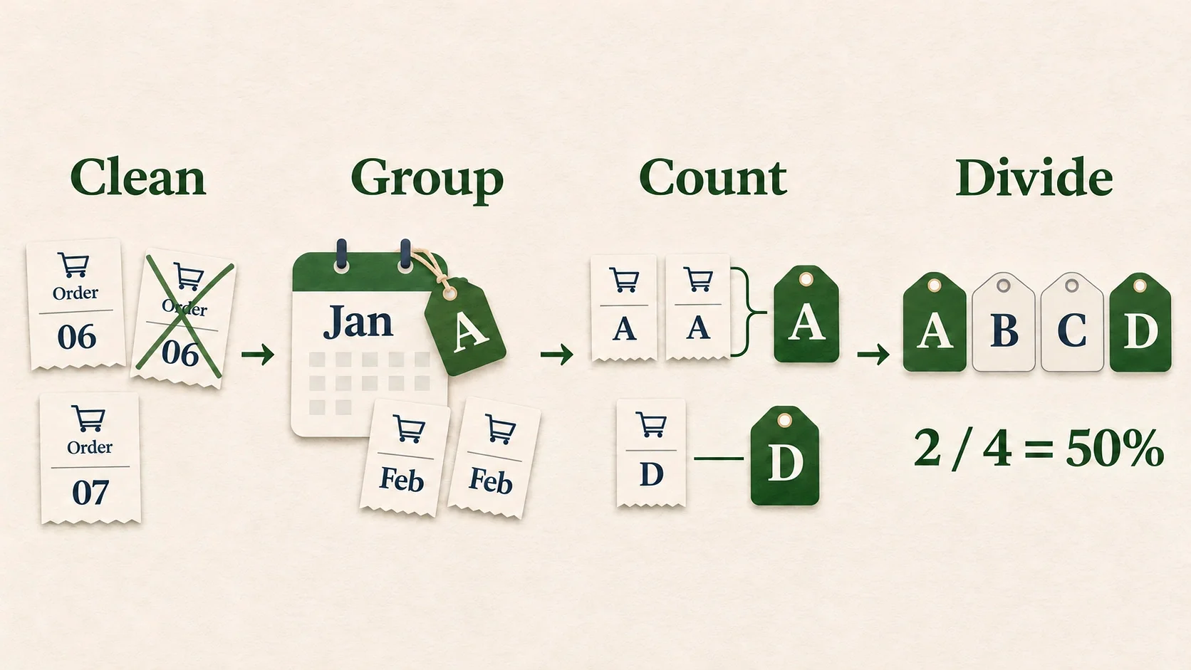
Build the table by choosing a return action, cleaning order records, assigning customers to their first-purchase month, and counting later purchasers. Divide each count by that cohort’s original size. Keep the rules beside the table so someone else can reproduce the result.
Step 1: choose the question and return action
Start with one question: what share of each first-purchase group buys again in each later calendar month?
For this example, a return means at least one eligible purchase during that month. A website visit or an email click doesn’t qualify. Those actions may be useful, but they answer different questions.
The records cover purchases through 31 March 2026. Assume complete earlier history, stable customer IDs, and one store timezone. In a real export, check those assumptions first; a customer’s first order in a short export may not be their first order with your business.
Step 2: decide which orders qualify
Write the purchase rule before counting. This example includes paid commercial orders and excludes cancellations, free replacements, and fully refunded orders. Remove identical duplicate order records; if two rows share an order ID but disagree, resolve the final order state before counting.
That is a chosen teaching rule, not a universal standard. A different refund policy can change both the starting group and later return counts, so document it and apply it consistently.
The sample starts with 22 records. Removing one duplicate, one cancellation, one replacement, and one fully refunded order leaves 18 eligible orders from nine customers.
Step 3: assign each customer to a starting month
Find each customer’s earliest eligible purchase and use its month as the cohort. Customer A first buys on 5 January, so A stays in January’s group after buying again in February and March.
The table below shows the eligible purchase dates. Every date falls in 2026; “none” means no eligible purchase in that month.
| Customer | January dates | February dates | March dates |
|---|---|---|---|
| A | 5, 20 | 10, 12 | 10 |
| B | 8 | None | 15 |
| C | 10 | None | None |
| D | 20 | 20 | None |
| E | None | 5 | 5 |
| F | None | 10 | None |
| G | None | 25 | 20, 22 |
| H | None | None | 2 |
| I | None | None | 20 |
January’s original group contains A, B, C, and D: four customers. February adds E, F, and G, while March adds H and I.
The excluded records don’t appear here. A duplicated February order is counted once; D’s March replacement and C’s fully refunded February order do not qualify under the stated rule.
Step 4: count distinct purchasers in each later month
For each group, count people who place at least one eligible order in a later month. Two orders from the same person still count as one returning purchaser for that period.
January Month 1: A and D buy again, so 2 ÷ 4 = 50%. A’s two February orders still count as one returning purchaser.
January Month 2: A and B buy, so 2 ÷ 4 = 50%. B skipped February and returned in March; absence in one month did not mean permanent loss.
February Month 1 is March. E and G buy again, giving two returning purchasers; G’s two March orders don’t make that count three.
Step 5: divide by the original cohort size
Use the same denominator for each period in a row:
Period repeat-purchase rate = distinct cohort customers purchasing in that period ÷ original cohort size × 100.
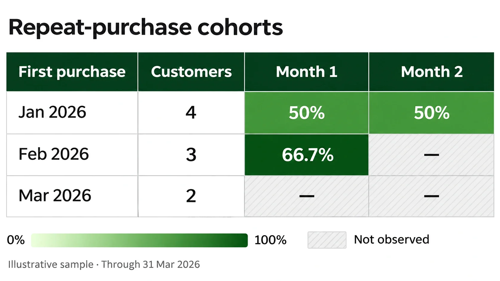
January’s denominator remains four, including customers who haven’t returned. February’s is three, so its Month 1 rate is 2 ÷ 3 × 100, or 66.7% after rounding.
| First-purchase cohort | Original customers | Month 1 | Month 2 |
|---|---|---|---|
| January | 4 | 2 of 4 (50%) | 2 of 4 (50%) |
| February | 3 | 2 of 3 (66.7%) | Not yet observed |
| March | 2 | Not yet observed | Not yet observed |
This table measures purchasing within each period. Keep that definition separate from other customer retention metrics, which may use different populations, starting events, or return rules.
How do you read the cohort table?
Read across a row to follow one starting group through time. Read down a column to compare groups at the same age. January’s Month 1 and February’s Month 1 cover different calendar months, but each is the month after that group’s first-purchase month.
Compare the same stage after acquisition
January has a 50% Month 1 rate; February has 66.7%. That is a fairer time comparison than comparing January’s March purchases with February’s March purchases, because the January group is one month older.
These are calendar-month buckets, not fixed 30-day windows. Someone who first buys on 31 January can enter Month 1 the next day. If your question is about buying again within 30 days, use a fixed-day calculation and wait until every included customer has had that full window.
Keep unobserved months blank
By 31 March, February’s group hasn’t reached Month 2 and March’s hasn’t reached Month 1. “Not yet observed” means the time hasn’t passed; zero would mean the period ended with no eligible purchases.
Don’t compare a partial current month with a complete earlier month. Record the observation cutoff so a reader knows which cells are finished.
Separate monthly returns from cumulative returns
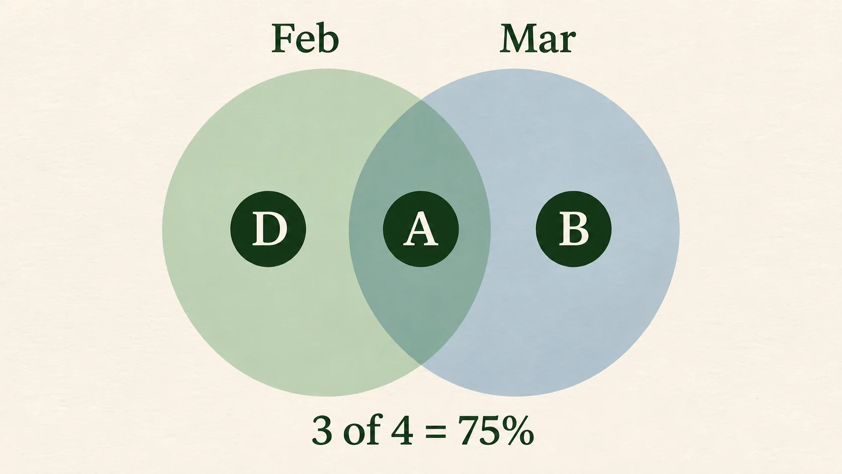
January cumulative repeat purchasing through Month 2 is different: A, B, and D have repeated at least once, so 3 ÷ 4 = 75%.
The monthly cells remain 50% and 50%, because different people can return in different months. Adding those percentages would count A twice.
Same-month repeat buying is another measure. A is January’s only same-month repeat purchaser, giving 1 ÷ 4 = 25%. Shopify’s customer-report documentation uses period 0 for returning orders within the first-order period, separately from first orders. Check a report’s definition before assuming its starting column must be 100%.
What mistakes change the answer?
Counting the wrong records or comparing unequal windows can change a cohort result without any change in customer behavior. In this sample, counting G’s March orders instead of G as one purchaser would inflate February’s return count from two to three. Check the records behind surprising cells.
Investigate an unexpected rate
If a customer-based rate exceeds 100%, inspect the numerator and denominator before interpreting it. Check for multiple orders counted as separate people, conflicting duplicate records, or customers assigned to more than one starting group.
An unexpected jump can also come from a changed purchase rule. Reconcile the included customer IDs against that rule, especially around refunds and replacements, before comparing the result with an earlier table.
Reading too much into small groups
One extra purchaser in February’s three-person cohort changes the rate by about 33 percentage points. Its 66.7% result cannot establish a healthy store benchmark.
Use the tiny sample to check the method. For a business decision, examine group sizes, purchase cycles, and patterns across several completed cohorts.
Treating a pattern as proof
A stronger cohort may coincide with a promotion, a new product mix, or a seasonal buying period. Its table doesn’t isolate which change caused the difference.
Check what changed, form a specific explanation, and decide how to test it. A cohort can point to the next question without answering why customers behaved that way.
How to do cohort analysis with AI for free
Use ChatGPT, Gemini, or Claude to analyze a small order file with explicit cohort rules. Start with the same 22-record example used above, ask for customer counts before a chart, and verify the calculations. A free account can help you try the method, but access and usage limits vary.
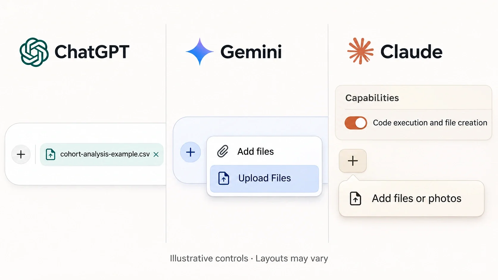
Generated illustration of the controls; layouts may vary.
Prepare one file before opening an AI tool
Use the illustrative cohort-analysis CSV to follow this walkthrough. It contains five columns: order_id, customer_id, order_date, order_type, and payment_status. Dates use year-month-day format, so 2026-03-05 means 5 March.
For your own orders, replace names and email addresses with stable customer labels before uploading. Keep the same label for every order from one person; replacing identifiers differently on each row would break the analysis. Review the service’s data settings before using business records.
Use one final record per order, with its payment and refund state resolved. Match your export to these five headers and map its status labels to your stated eligibility rule; ask the AI to flag uncertain mappings rather than guess.
Don’t upload just a screenshot of a sales chart. The tool needs the order rows to assign customers and count returns.
Copy this cohort-analysis prompt
The prompt fixes the definition before the AI starts calculating. Use it unchanged with the sample CSV; for your own data, update the cutoff and verify that the history is complete enough to identify first purchases.
Analyze the attached illustrative order CSV. Its columns are order_id, customer_id, order_date, order_type, and payment_status.
The sample has complete purchase history through the end of 2026-03-31, with no earlier orders. Dates are already in one store timezone. Exclude records after that cutoff before assigning cohorts or counting returns.
Remove identical duplicate records by order_id. If records with the same order_id disagree, flag them and ask how to resolve the final order state; do not keep an arbitrary row.
Include only rows where order_type is sale and payment_status is paid; exclude cancelled orders, fully_refunded orders, and replacements. Show how many rows each rule removes, then show eligible order and customer counts.
Assign each customer once to the calendar month of their earliest eligible purchase. For each cohort, show its original customer count and distinct purchasers in Month 1 and Month 2. Month 1 means the next calendar month, not the next 30 days.
Count a person once per period, even if they place several orders. Divide by the original cohort size.
Only fill periods whose calendar month has ended by the cutoff. Leave incomplete or future periods blank; do not fill them with zero.
Return the cleaned orders, customer-to-cohort assignments, purchaser counts, and percentage table. Use computation when available and explain the calculation method. Flag missing fields or ambiguity instead of guessing. Do not predict future retention or claim that a campaign caused a result.
Choose one tool below, sign in to its free account, and start a new chat. Attach the sample using that tool’s controls, then send the prompt above with it. There is no need to run the same file through all three tools.
How to do cohort analysis with ChatGPT
Open ChatGPT and drag the CSV into the message box. Wait for the attachment to appear before sending the shared prompt, so the request includes the actual order file.
ChatGPT’s free-tier documentation includes data analysis and uploads, with separate tool limits. Its analysis guide recommends clear column names and reviewing the method and outputs. If your free allowance is exhausted, wait for access to return; a paid plan isn’t part of this walkthrough.
How to do cohort analysis with Gemini
Open Gemini. Beside the prompt box, select Add files → Upload Files and choose the CSV from your device. Once it is attached, paste the shared prompt and select Submit.
Google documents the file-upload steps and access without a Google AI plan. Free access has limits, and account availability can vary. Keep the full history needed for the question rather than trimming older orders just to fit an upload.
How to do cohort analysis with Claude
Open Claude. In Settings → Capabilities, check that Code execution and file creation is enabled; an updated layout may call it Create and edit files. This enables the file-analysis workflow described here.
In the chat box, select + → Add files or photos, choose the CSV, and select Open. Send the shared prompt once the file is attached.
Claude documents both the attachment steps and file-analysis capability for Free accounts. Analysis and file creation use the account’s allowance; they aren’t unlimited.
Check the AI result before using it
With this sample, the output should reconcile to 18 eligible orders from 9 customers, with starting groups of 4, 3, and 2. January’s Month 1 and Month 2 should each show 2 returning purchasers and 50%; February’s Month 1 should show 2 and 66.7%.
Ask the tool to explain any mismatch using individual customer IDs. A heatmap with the right colors is still wrong if it counts A’s two February orders as two people.
Also check January’s cumulative repeat rate separately: it is 75% through Month 2, not the sum of its monthly rates. Never turn a missing future period into a zero just to finish a chart.
If the reply skips the working, use this follow-up in any of the three tools:
Show the cleaned rows, customer-to-cohort assignments, and distinct customer IDs behind each monthly count. Explain any mismatch with the expected sample results before changing the table.
Once the counts agree, ask for the output you can keep:
Provide the cohort counts and percentages as a downloadable CSV and a heatmap. Label unobserved periods separately from zero. If you cannot create a download, return CSV text that I can copy into a spreadsheet.
Which repeat-purchase question should you investigate next?
Choose one starting group, one return action, and one complete time window. Then identify the decision the comparison could change: when to investigate a weak second-purchase month, for example, or whether a particular acquisition period deserves a closer look.
Putler does not currently offer cohort analysis. The example here explains a method; it isn’t a report generated in Putler.
Before sharing your own table, write its purchase rule and cutoff beside it. Ask another person to trace one cell back to the underlying customers, just as January’s 50% cells trace back to two of its four original buyers.
FAQ
What is a customer cohort?
A customer cohort is a group defined by a shared starting point or condition. In this guide, customers who make their first eligible purchase in the same calendar month form one cohort. Their membership stays fixed while later purchases are measured over time.
How do you read a cohort table?
Read across a row to follow one group as it ages and down a column to compare groups at the same stage. Check the metric definition, original group size, and observation cutoff first. An unobserved future period is different from a completed period with zero purchases.
How is cohort analysis different from retention rate?
A retention rate summarizes continued activity under a defined rule. Cohort analysis separates starting groups and follows each one through time. It can reveal differences hidden in an overall rate, provided the groups use consistent definitions and have had equal time to complete the compared period.
Can you start cohort analysis in a spreadsheet?
Yes. A small, clean order history can support a first-purchase cohort table. You’ll need stable customer identifiers, order dates, eligibility rules, and enough history to identify first purchases. Count distinct purchasers per period, document the denominator, and check a few cells against individual records before relying on the result.
Can AI do cohort analysis for free?
ChatGPT, Gemini, and Claude offer free access that can help analyze a small order file, subject to their current tool and usage limits. Supply the cohort definition, eligible-order rule, and observation cutoff. Check the customer assignments and counts yourself before treating the resulting table as useful business evidence.